

A century ago engineers had very good and robust means of drafting 2D curves using specialized spline sets and curve templates (e.g. French curves). But these proved difficult to replicate in early computers; the need for fast, simple algorithms drove first Bezier, and then de Boor to embrace the idea of polynomial-based splines.
Creating a spline from independent polynomial functions along the x/y/z axes has a number of problems. Such splines cannot be represented in arc length form and, more importantly, controlling their curvature functions is not easy. Polynomial splines are computationally simple but mathematically complex.
Computing power has greatly improved since the late 60s when the modern suite of polynomial curves were created and we can now numerically solve the kind of curves engineers used before computers (and still use to today for road network design, high speed rail, etc): clothoids.
Clothoids

A better way to do splines is to start with a curvature function with the properties you want and integrate backwards. For example in civil engineering the three basic shapes are classical clothoids (whose curvature function is linear), circular arcs (constant curvature) and lines (zero curvature). Since these are all linear functions we can represent all three with a spline whose curvature function is simple linear interpolation:
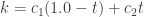
Where 


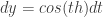
To integrate it in 2D, all we do is plug it into the following formula:

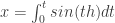

Note that 


So we now have a curve whose curvature starts at
So now we have a function that takes two spatial points, 

But this isn’t good enough. We want to string several of these curves together, and we want to enforce constraints at shared vertices: tangential continuity, curvature continuity, whatever we want. For basic G2 continuity we have six constraints at the endpoints of each curve segment: the segment must span two points in space, have shared tangents with adjacent curves and shared curvatures. We’ve eliminated two of these constraints by how we’ve formulated the curve, leaving us with four. This leads us to Raph Levien’s idea of using a cubic polynomial for our curvature function. It doesn’t matter what form the polynomial takes; I like to use 1D Beziers myself, but you also use a four-segment piecewise-linear function if you want.
We can represent the cubic like this:


Which is the “intuitive” form of the Bezier polynomial. One can also use more traditional Bernstein basis functions to get the same equation:


Or we could dispense with interpolation formulas entirely and just use a raw cubic:

I like the Bezier (Bernstein) form as the curvature at the endpoints is equal to the first and last coefficients.
Numerical Integration
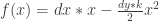
Integrating this curve isn’t terribly difficult. This is due to a nice property of arc-length parameter curves, where every point in


Thus, the higher derivatives are all functions of the first derivative the curvature function and its derivatives. This makes it easy to construct a Taylor approximation.

Quadrature
However, a simple Taylor approximation will not work. We need to use it in a quadrature. For example, we might do something like this bit of python code:
def quadrature(t):
  steps = [some number of steps, e.g. 5]
  s = 0
  ds = t / steps
  x = 0
  y = 0

  for i in range(steps):
    k = curvature(s)
    th = [integral of k]

    dx = sin(th)
    dy = cos(th)

    x += dx*ds - 0.5*dy*ds*ds
    y += dy*ds + 0.5*dx*ds*ds

    s += ds
  return [x, y]
This might be wrapped in another function, that fits the clothoid between points p1 and p2:
def getpoint(t, p1, p2):
  start = quadrature(0.0)
  end = quadrature(1.0)
  vector = end - start

  angle = atan2(vector.y, vector.x)
  scale = length(p1 - p2) / length(vector)

  p = quadrature(t) - start
  p = rotate(p, angle)
  p = scale(p, scale)
  p = p + p1;

  return [p.x, p.y, scale, angle]
Practical Splines
Now it’s time to build a spline out of these curves. To do so we need some way of maintaining continuity of the vertices. The idea is to build a list of constraints, e.g. tangent constraint, curvature constraint, etc (see page 119 of Raph Levien’s phd thesis). Then use any non-linear constraint solver to solve them. The number of parameters in the curvature function should be equal to the maximum number of constraints.
Each constraint outputs an error value. For example, a tangent constraint would take two segments, and return the angle between the tangents at their shared vertex. A curvature constraint would return the difference between the curvatures at the vertex (made sure to put the curvature in global space by dividing by the scale that was returned in getpoint).
For a non-linear constraint solver, you can use pretty much anything. I like to use a modified version of the Geiss-Seidal solver from this game physics paper. It’s very flexible and doesn’t require that the number of constraints and parameters perfectly match. Raph Levien uses a simple Jacobian method of multiplying the parameters by the inverse of the constraint matrix Jacobian.
Results
What you get is a nice, pretty looking spline that’s incredibly versatile. It’s useful for everything from designing high-speed rail networks to vector graphics to even 2D animation.

Prologue: Why “Modern” Polynomial Splines Suck
It’s funny. A hundred years ago engineers had a perfectly good, mathematically robust means of drafting curves. Curvature was easy to control, with specialized spline sets and curve templates (e.g. French curves) that made smooth curved shapes easy to make.
And then Bezier came on the scene, followed by de Boor, and set engineering drafting back to the dark ages. Modern computers can replicate the robustness and ease of traditional drafting tools, but this wasn’t true at the dawn of CAD in the late 60s. The need for fast, simple algorithms drove first Bezier, and then de Boor to embrace the idea of polynomial-based splines.
Simple polynomial splines have an enormous number of problems. They can’t be represented in arc length form. It is extremely difficult to control their curvature, which is often “wavy.” But most of all it just doesn’t make sense mathematically to split curves into independent x, y, and z functions.
Traditional drafting understood this. The wooden splines of old guaranteed curvature continuity in a way that’s very difficult to do with simple polynomials today. Curve templates were based on the “ideal elastica”, which was alternatively called the clothoid, the Cornu spiral, the Euler spiro, and the French curve (in the art world).
