
Sampling is the bane of computer graphics. Aliasing, accuracy, and noise must all be traded off against each other. A sampling method that works well for low sample counts might be inferior at high sample counts.
As an example of the sort of problem sampling is meant to solve, take this simple grid:
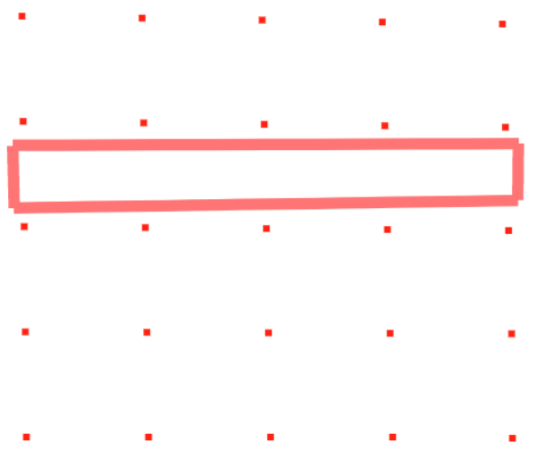
None of the red points fall inside the red rectangle. This is known as aliasing. We can mitigate this by adding noise to the sampling points:
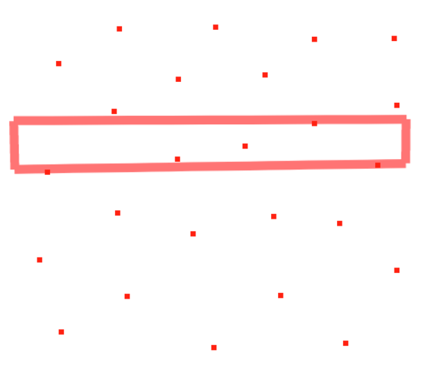
Now some of the red sampling points do fall within the red rectangle (I know, I know, I should have picked contrasting colors). But how do we “add noise” exactly? This is actually a fairly difficult problem in computer graphics. Let’s look at another problem, image stippling. Say we want to render an image entirely in black and white (no grey). To do so we compare every pixel in the image with a mask. If the pixel is brighter than the mask value we make it white, otherwise we make it black.
What should this mask look like? If we use uniform white noise, the results are terrible:

The stippling mask is in the top right corner (it’s tiled across the image). Luckily there is another, better type of noise: blue noise.
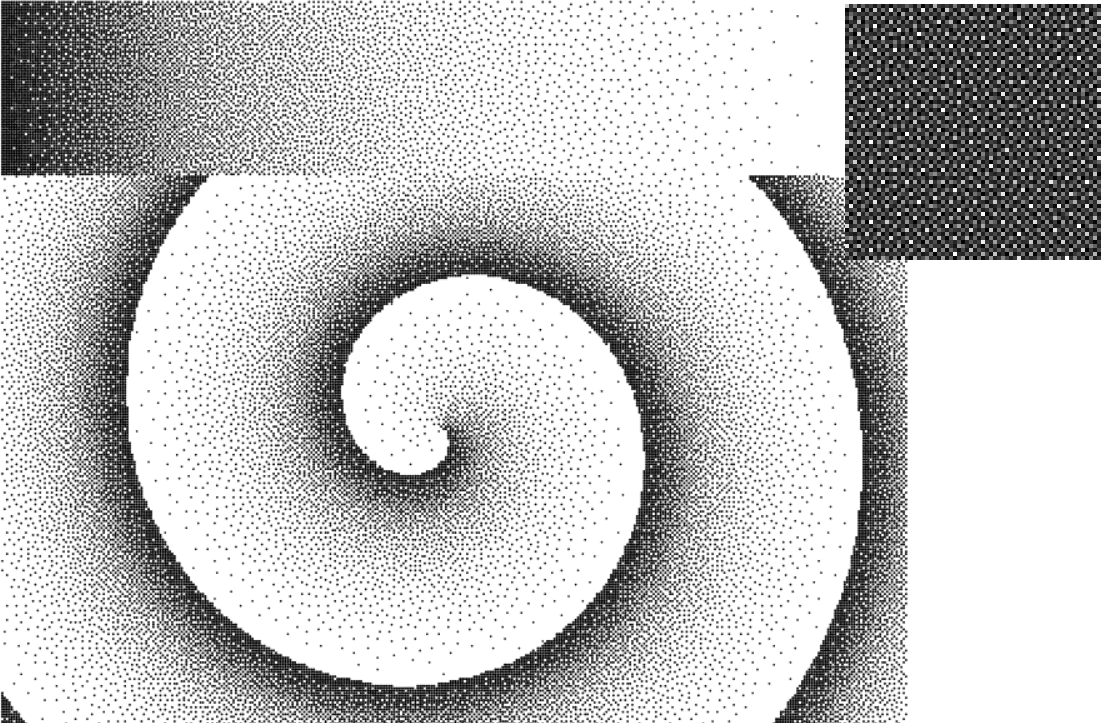
Much better! The mask in the upper right corner was generated using the “void and cluster” method, originally developed for the printing industry. Void and cluster generates so-called “blue noise”, with a 2D Fourier spectrum that looks like this:
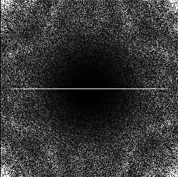
The line in the middle is a bug in my FFT code. There aren’t many good FFT libraries in JavaScript, my preferred language for prototyping research stuff. I could have used a DFT, but that would have been too slow for what I’m doing.
As you can see, the high frequencies in the middle are suppressed. This makes nice, visually pleasing noise patterns that aren’t too noticeable.
Methods for generating blue noise generally fall under two categories: ones that generate simple point sets and ones that generate progressive point sets suitable for image stippling, importance sampling in ray tracing, etc. Void and cluster falls under the latter category.
A lot of research has been done on generating simple point sets with blue noise properties, but virtually no research has been done for progressive sets since the 90s. An important exception is Wei’s Multi-Class Blue Noise Sampling, published in 2010. Playing around in this area is one of my hobbies. One of the challenges is simply to know what’s possible to achieve in terms of sampling properties. It’s relatively simple to make progressive blue noise sets in 2D; void-and-cluster is a pretty simple algorithm. As explained in this excellent blog post, however, things get more complicated in 3D. For higher dimensional noise it’s often desirable that the blue noise property hold in lower dimensions as well as higher ones. As explained in the blog post, this isn’t possible as a general matter. Trade-offs must be made.
Blue noise methods typically work by either enforcing a set of constraints or minimizing some function, but another method is to transform a uniform white noise distribution into blue noise by targeting the frequency spectra directly. This is actually how the first progressive blue noise algorithm, the predecessor to void-cluster, worked. It’s very computationally intensive and not very practical in higher dimensions, but it can help explore different Fourier spectra.
It’s pretty difficult to optimize the Fourier spectrum of point sets that aren’t aligned with a grid, mostly because there aren’t any FFT algorithms for this purpose (that I know off) and normal DFT is pretty slow. But if we restrict ourselves to void-cluster-style progressive point sets that generate points inside of grids then a really simple algorithm suggests itself:
- Fill a grid (2D or otherwise) with white noise.
- Compute the FFT.
- Randomly swap some points.
- Computer the FFT again. If the new FFT spectrum is closer to our target spectrum than the old one, keep the swapped points and the new FFT. Otherwise, unswap them and keep the old FFT.
- Repeat from 3 until convergence.
Here’s an example of the output of this process, scaled up 4x:
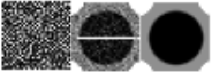
The target FFT is on the right, the generated point set is on the right and its FFT is in the middle. As you can see, the target FFT is a bit weird, and the point set isn’t terribly good, but that’s what this method is for: to see what sort of noise is generated by different FFT spectra and what sort of trade-offs we can make.
This is especially useful in 3D:

Here we have four sets of slices of a 16×16 noise set and it’s associated FFTs. The top left is the 3D target FFT. The top right is the generated noise. The bottom left is the noise’s 3D FFT, while the bottom right are 2D FFTs for each slice of the noise along the X axis.
Versatile, eh? One must love brute-force stochastic optimization. So easy. Of course this method suffers from the “curse of dimensionality” like no other, but it’s not really meant for practical use, it’s just to see what’s possible.
Anyway, I plan on publishing the code for this soon, so watch out for that. Note that the patent on generating blue noise via FFT optimization recently expired, so no need to worry about that (I don’t even know if it would have covered my method or not, I’m not a patent lawyer).
